Simulating flux from casks

As described in the introduction, the main goal of this package is to simulate the antineutrino flux emitted by spent nuclear fuel (SNF) casks. This is done using two main classes: Spectrum and Cask, which are defined in the snf_simulations.spec and snf_simulations.cask modules, respectively.

Once we’ve created a Cask object, we can use the get_total_spectrum method to create a Spectrum object representing the combined antineutrino spectrum from all isotopes in the cask.

from snf_simulations.cask import Cask

# Create a Cask object for 100 kg of SNF from the Sizewell reactor
reactor = "sizewell"
mass = 10000  # 10 tonnes
cask = Cask.from_reactor(reactor, total_mass=mass)
print(cask)

removal_time = 0.5  # years
total_spec = cask.get_total_spectrum(removal_time=removal_time)
print(total_spec)

<Cask "sizewell_cask", total_mass=10000 kg>
<Spectrum "sizewell_cask total spectrum", energy_range=(0.0-5313.0 keV)>

Measuring the flux at a distance

We can get a measure for the total antineutrino flux above a given energy threshold by integrating the the total spectrum. For inverse beta decay the threshold is 1.806 MeV, so we integrate above this energy to get the total flux of antineutrinos that can be detected.

total_flux = total_spec.integrate(lower_energy=1806)
print(f"Total flux above 1.806 MeV: {total_flux:.3e} per second")

Total flux above 1.806 MeV: 2.397e+17 per second

This is the total flux emitted in all directions. To get the flux at a given distance from the cask, we can then use the calculate_flux_at_distance function from the snf_simulations.physics module, which takes the total flux and the distance as arguments. It calculates the flux using the inverse square law:

\[F(d) = \frac{F_{tot}}{4 \pi d^2}\]

where \(F(d)\) is the flux at distance \(d\), and \(F_{tot}\) is the total flux emitted by the cask isotropically.

from snf_simulations.physics import calculate_flux_at_distance

distance = 40  # meters
flux_at_40m = calculate_flux_at_distance(total_flux, distance)

print(
    f"Single {cask.total_mass / 1000:.0f}-tonne {reactor.capitalize()} cask "
    f"at {distance}m after {removal_time} years:"
)
print("Antineutrino flux:")
print(f"  {flux_at_40m:.3e} per cm2 per second")
print(f"  {flux_at_40m * 60 * 60 * 24:.3e} per cm2 per day")

Single 10-tonne Sizewell cask at 40m after 0.5 years:
Antineutrino flux:
  1.192e+09 per cm2 per second
  1.030e+14 per cm2 per day

Simulating events in a detector

Finally, we can calculate how that flux would convert into the number of events in our detector using the calculate_event_rate function.

Note

At the moment only the VIDARR detector is supported. See this GitHub Issue for details.

from snf_simulations.physics import calculate_event_rate

rate_lower, rate_upper = calculate_event_rate(flux_at_40m, 0.2, 0.4)
print("Event rate in VIDARR detector:")
print(f"  {rate_lower:.3e} to {rate_upper:.3e} per second")
print(f"  {rate_lower * 60 * 60 * 24:.3f} to {rate_upper * 60**2 * 24:.3f} per day")

Event rate in VIDARR detector:
  1.773e-07 to 3.547e-07 per second
  0.015 to 0.031 per day

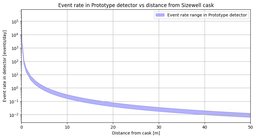
We can plot how the event rate varies with distance from the cask.

import matplotlib.pyplot as plt
import numpy as np

# Get a range of distances
distances = np.concatenate(([0.01, 0.05, 0.1, 0.5], np.linspace(1, 50, 50)))
removal_time = 0.5  # years

total_spec = cask.get_total_spectrum(removal_time=removal_time)
total_flux = total_spec.integrate(lower_energy=1806)
event_rates = []
for distance in distances:
    flux_at_distance = calculate_flux_at_distance(total_flux, distance)
    rate_lower, rate_upper = calculate_event_rate(flux_at_distance, 0.2, 0.4)
    event_rates.append((rate_lower * 60 * 60 * 24, rate_upper * 60 * 60 * 24))
event_rates = np.array(event_rates)

figure = plt.figure(figsize=(10, 5))
axes = figure.add_subplot(1, 1, 1)
axes.fill_between(
    distances,
    event_rates[:, 0],
    event_rates[:, 1],
    color="blue",
    alpha=0.3,
    label="Event rate range in VIDARR",
)
axes.set_xlim(0, 50)
axes.set_xlabel("Distance from cask [m]")
axes.set_ylabel("Event rate in VIDARR [events/day]")
axes.set_title(
    f"Event rate in VIDARR detector vs distance from {reactor.capitalize()} cask"
)
axes.set_yscale("log")
axes.grid()
axes.legend()

plt.show()

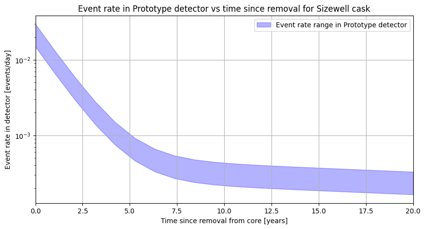
Or we could plot how the event rate varies with time after removal from the reactor.

removal_times = np.linspace(0, 20, 20)  # years
distance = 40  # meters

event_rates = []
for removal_time in removal_times:
    total_spec = cask.get_total_spectrum(removal_time=removal_time)
    total_flux = total_spec.integrate(lower_energy=1806)
    flux_at_distance = calculate_flux_at_distance(total_flux, distance)
    rate_lower, rate_upper = calculate_event_rate(flux_at_distance, 0.2, 0.4)
    event_rates.append((rate_lower * 60 * 60 * 24, rate_upper * 60 * 60 * 24))
event_rates = np.array(event_rates)

figure = plt.figure(figsize=(10, 5))
axes = figure.add_subplot(1, 1, 1)
axes.fill_between(
    removal_times,
    event_rates[:, 0],
    event_rates[:, 1],
    color="blue",
    alpha=0.3,
    label="Event rate range in VIDARR",
)
axes.set_xlim(0, 20)
axes.set_xlabel("Time since removal from core [years]")
axes.set_ylabel("Event rate in VIDARR [events/day]")
axes.set_title(
    f"Event rate in VIDARR detector vs time since removal "
    f"for {reactor.capitalize()} cask"
)
axes.set_yscale("log")
axes.grid()
axes.legend()

plt.show()